Shapefiles - Of avalanches and ibexes · Blog

At Liip, we recently completed an application for architecture students that uses shapefiles as its backbone to deliver information about building plots in the city of Zurich. They are displayed on a map and can be inspected by users. A similar project was done by a team of students, of which I was part, for the FHNW HT project track: a fun-to-use web application that teaches children in primary school about their municipality.

But shapefiles can do more than help to enhance the user experience – they also contain data that, when brought into context, yield interesting insights. So let's see what I can find out by digging into some shapefiles and building a small app to explore them.
In this blog post, I will take a practical approach to working with shapefiles and show you how to get started with them!

Alpine Convention

The first hurdles in working with shapefiles are understanding what they actually are and acquiring them in the first place.

Shapefiles are binary files that contain geographical data. They usually come in groups of at least three different files having the same name, their only difference is their file extension: .shp, .shx and .dbf. However, a complete data set can contain many more files. The data format was developed by Esri and introduced in the early 1990s. Shapefiles contain what are known as features, namely a geometrical shape with its metadata. A feature could be a point (single X/Y coordinates) and a text explaining what this point is, or a polygon consisting of several X/Y points, a single line, multiple lines, etc.

To get shapefiles to work with, I took a look at OpenData.swiss. OpenData offers a total of 102 different shapefile data sets (as of November 2017). All I have to do is download and start to work with them. For this example, I chose a rather small shapefile: Alpine Convention consisting of the perimeters of the Alpine Convention in Switzerland.
Since these files are binaries and I cannot look at them in a text editor, I needed a tool to look at what I just downloaded.

Introducing QGIS – a free and open-source geographic information system

QGIS is an extensive solution for all kinds of GIS. It can be downloaded and installed for free, and has a lot of plugins and an active community. I'm going to use it to have a look at my previously downloaded shapefile.
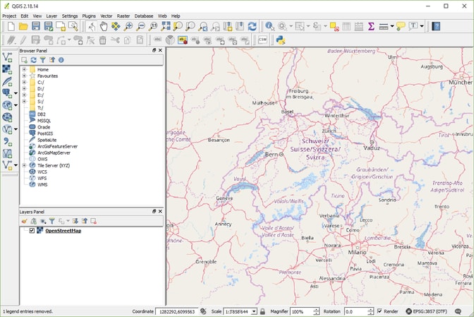
For this example, I installed QGIS with the OpenLayers plugin. This is what it looks like when started up:

To gain a reference point for where I actually am and where my data goes, I add OpenStreetMap as a layer. I also pan and zoom the map to focus onSwitzerland.

The next step would be to actually open the shapefile, so QGIS can display it on top of the map. For that I can simply double-click the .shp file in the file browser.

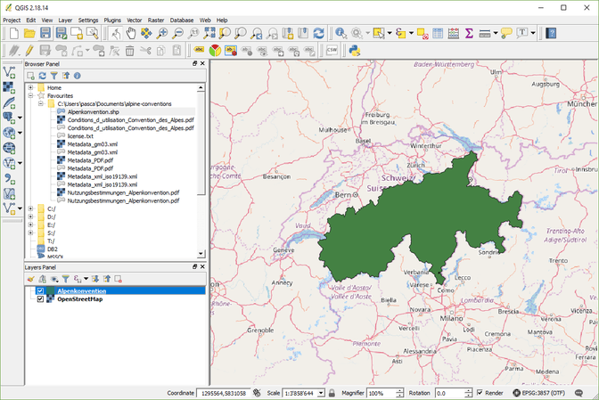
This provides some information about the shapefile I'm dealing with already. What area it covers, and how many features there are. The Alpine Convention shapefile seems to only consist of one feature, a big polygon, which is enough, given that it only shows the perimeters of the Alpine Convention in Switzerland.

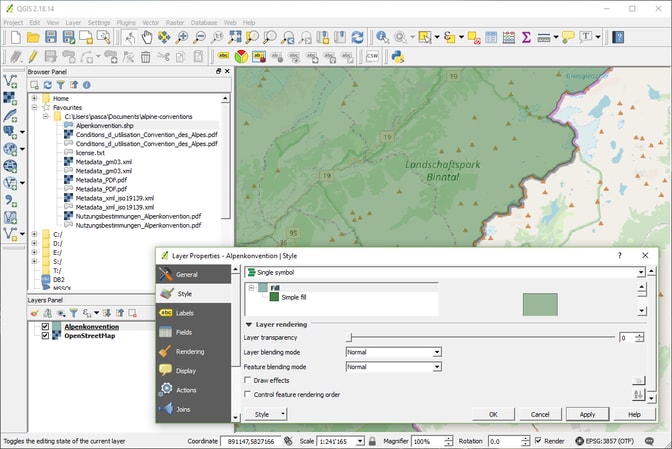
To see the areas and/or details it covers, I can alter the style of the layer and make it transparent.There is the possibility to zoom in more and see the shape is accurate. Its edges should exactly cover the Swiss borders.

Marvelous. Now that I've seen the shape of the feature, I'll have a look at the metadata the shapefile offers. They can be inspected by opening the attributes table of the shapefile in the bottom left browser.

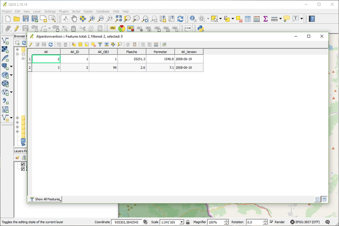
This file doesn't offer much metadata, but now I can see that there are two features. In any case, there might be more interesting shapefiles out there to work with.
But I'm going to stick with the Alpine topic.

Of avalanches and ibexes

Digging through OpenData's shapefile repository a bit further, I found two more shapefiles that could potentially yield interesting data: the distribution of ibex colonies and the state of natural hazard mapping by municipalities for avalanches.

As awesome as QGIS is for examining the data at hand, I want to build my own explorer, maybe even one built upon multiple shapefiles and in my own design. For this, there's multiple libraries for all kinds of languages. For web development, the three most interesting ones would be for PHP, https://pypi.python.org/pypi/pyshptext Python and JavaScript.

For my example, I'll build a small frontend application in JavaScript to display three shapefiles: the Alpine Convention, the ibex colonies and the avalanche mapping. For this I'm going to use a JavaScript package simply called "shapefile" and Leaflet.js to display the polygons from the features. But first things first.

Reading the features

Disclaimer: the following code examples are using ES6 and imply a webpack/babel setup. They're not exactly copy/paste-able, but they show how to work with the tools at hand.
First, I try to load the Alpine Convention shapefile and log it into the console. The shapefile package mentioned above comes with two examples in the README, so for simplicity, I just roll with this approach:

import { open } from 'shapefile'

open('assets/shapefiles/alpine-convention/shapefile.shp').then(source => {
  source.read().then(function apply (result) { // Read feature from the shapefile
    if (result.done) { // If there's no features left, abort
      return
    }

    console.log(result)

    return source.read().then(apply) // Iterate over result
  })
})

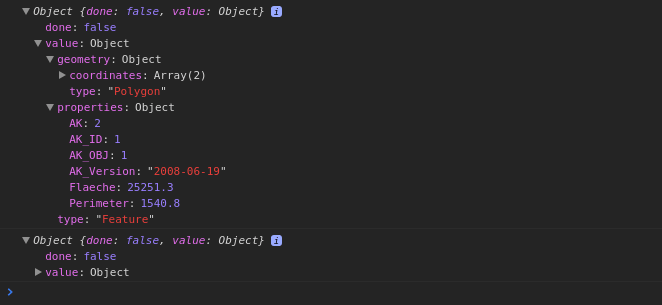
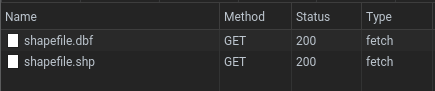
Works like a charm! This yields the two features of the shapefile in the console. What I see here, is that the properties of each feature, normally stored in separate files, are already included in the feature. This is the result of the library fetching both files and processing them:

Now I have a look at the coordinates that are attached to the first feature. The first thing that occurs is that there's two different arrays, implying two different sets of coordinates, but I'm going to ignore the second one for now.

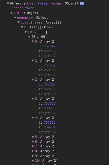
And there's the first pitfall. These coordinates look nothing like WGS84 (latitude/longitude). Coordinates in WGS84 should be a floating-point number, ideally starting with 47 and 8 for Switzerland, so this shapefile meant I was dealing with a different coordinate reference system (or short: CRS). In order to correctly display the shape on top of a map or use it with other data, I would want to convert these coordinates to WGS84 first, but in order to do that, I need to figure out which CRS this shapefile is using. Since this shapefile comes from the Federal Office for Spatial Development ARE, the CRS used is most likely CH1903, aka the "Swiss coordinate system".

So in order to convert that, I need some maths. Searching the web a bit, I found a JavaScript solution to calculate back and forth between CH1903 and WGS84. But I only need some parts of it, so I copy and alter the code a bit:

// Inspired by https://raw.githubusercontent.com/ValentinMinder/Swisstopo-WGS84-LV03/master/scripts/js/wgs84_ch1903.js

/**
 * Converts CH1903(+) to Latitude
 * @param y
 * @param x
 * @return {number}
 * @constructor
 */
const CHtoWGSlat = (y, x) => {
  // Converts military to civil and to unit = 1000km
  // Auxiliary values (% Bern)
  const yAux = (y - 600000) / 1000000
  const xAux = (x - 200000) / 1000000

  // Process lat
  const lat = 16.9023892 +
    (3.238272 * xAux) -
    (0.270978 * Math.pow(yAux, 2)) -
    (0.002528 * Math.pow(xAux, 2)) -
    (0.0447 * Math.pow(yAux, 2) * xAux) -
    (0.0140 * Math.pow(xAux, 3))

  // Unit 10000" to 1" and converts seconds to degrees (dec)
  return lat * 100 / 36
}

/**
 * Converts CH1903(+) to Longitude
 * @param y
 * @param x
 * @return {number}
 * @constructor
 */
const CHtoWGSlng = (y, x) => {
  // Auxiliary values (% Bern)
  const yAux = (y - 600000) / 1000000
  const xAux = (x - 200000) / 1000000

  // Process lng
  const lng = 2.6779094 +
    (4.728982 * yAux) +
    (0.791484 * yAux * xAux) +
    (0.1306 * yAux * Math.pow(xAux, 2)) -
    (0.0436 * Math.pow(yAux, 3))

  // Unit 10000" to 1 " and converts seconds to degrees (dec)
  return lng * 100 / 36
}

/**
 * Convert CH1903(+) to WGS84 (Latitude/Longitude)
 * @param y
 * @param x
 */
export default (y, x) => [
  CHtoWGSlat(y, x),
  CHtoWGSlng(y, x)
]

And this I can now use in my main app:

import { open } from 'shapefile'
import ch1903ToWgs from './js/ch1903ToWgs'

open('assets/shapefiles/alpine-convention/shapefile.shp').then(source => {
  source.read().then(function apply (result) { // Read feature from the shapefile
    if (result.done) { // If there's no features left, abort
      return
    }

    // Convert CH1903 to WGS84
    const coords = result.value.geometry.coordinates[0].map(coordPair => {
      return ch1903ToWgs(coordPair[0], coordPair[1])
    })

    console.log(coords)

    return source.read().then(apply) // Iterate over result
  })
})

Which yields the following adjusted coordinates:

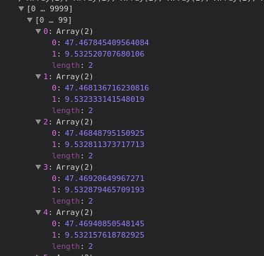
A lot better. Now I'll throw them on top of a map, so I have something I can actually look at.

Making things visible

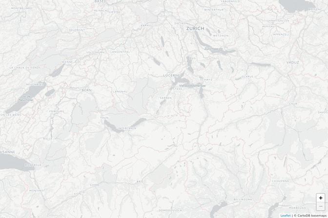
To do so, I added Leaflet to the app together with the Positron (lite) tiles from CartoDB. The Positron (lite) theme is light grey/white, which provides a good contrast to the features I'm going to display over them. OpenStreetMap is awesome, but too colourful, so the polygons are not visible enough.

import leaflet from 'leaflet'
import { open } from 'shapefile'
import ch1903ToWgs from './js/ch1903ToWgs'

/**
 * Add the map
 */
const map = new leaflet.Map(document.querySelector('#map'), {
  zoomControl: false, // Disable default one to re-add custom one
}).setView([46.8182, 8.2275], 9) // Show Switzerland by default

// Move zoom control to bottom right corner
map.addControl(leaflet.control.zoom({position: 'bottomright'}))

// Add the tiles
const tileLayer = new leaflet.TileLayer('//cartodb-basemaps-{s}.global.ssl.fastly.net/light_all/{z}/{x}/{y}.png', {
  minZoom: 9,
  maxZoom: 20,
  attribution: '&copy; CartoDB basemaps'
}).addTo(map)

map.addLayer(tileLayer)

/**
 * Process the shapefile
 */
open('assets/shapefiles/alpine-convention/shapefile.shp').then(source => {
  source.read().then(function apply (result) { // Read feature from the shapefile
    if (result.done) { // If there's no features left, abort
      return
    }

    // Convert CH1903 to WGS84
    const coords = result.value.geometry.coordinates[0].map(coordPair => {
      return ch1903ToWgs(coordPair[0], coordPair[1])
    })

    console.log(coords)

    return source.read().then(apply) // Iterate over result
  })
})

This already shows me a nice looking map I can work with:

The next step is to hook up the map with the shapefile loading. For this, I create Leaflet polygons out of the coordinates I transformed to WGS84 earlier:

// ...

// Convert CH1903 to WGS84
const coords = result.value.geometry.coordinates[0].map(coordPair => {
  return ch1903ToWgs(coordPair[0], coordPair[1])
})

const leafletPolygon = new leaflet.Polygon(coords, {
  weight: 0.5,
  color: '#757575',
  fillOpacity: 0.3,
  opcacity: 0.3,
})

leafletPolygon.addTo(map)

// ...

And I have a look at the result:

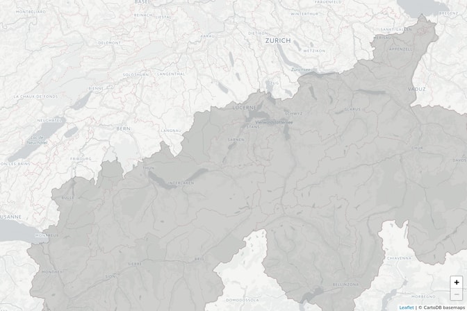
Nice!

The end result

With more UI and adding a toggle for the multiple shapefiles I downloaded earlier, I can build a little app that shows me the hazard zones for avalanches and where ibexes are living in Switzerland:

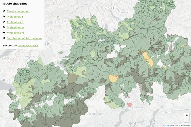
We can see the two shapefiles in action: the light green, green, yellow and red polygons are municipalities with some risk of avalanches (light green = low, green = mid-low, yellow = mid, red = high), the darker polygons on top are the ibex colonies.

This map already offers good insights on the behaviour of ibexes: apparently they only live in low-hazard to mid-low-hazard zones for avalanches. They also tend to avoid mid-hazard and high-hazard zones. Since ibexes prefer alpine terrain and such terrain usually bears some danger of avalanches, this is plausible, but now I've got some visible data to actually support this claim!

The finished app can be found in action here, and its source code can be found in this repository.

The pitfalls

Although shapefiles are a powerful way to handle GIS data, there are some pitfalls to avoid. One I've already mentioned is an unexpected CRS. In most cases, it can be identified at the point of usage, but checking which CRS a shapefile uses when inspecting it is recommended. The second big pitfall is the size of the shapefiles. When using some shapefiles with JavaScript in the browser directly, the browser might crash while trying to handle the huge amount of polygons. There are several solutions, though: you can either simplify the shapefile by removing unnecessary polygons or pre-process it and store its polygons in some kind of database and only query the polygons currently in sight.

Takeaway thoughts

Personally, I love working with shapefiles. There's a lot of use cases for them and exploring the data they hold is something really exciting. Even though there might be a pitfall or two, in general it's a piece of cake, as you can get something up and running with little effort. The OpenData community uses shapefiles quite a lot, so it is a well-established standard and there's a lot of libraries and tools out there that make working with shapefiles as awesome as it is.

Do you have a question, a comment, or just feeling inspired? Mention us or share this article on Mastodon, Twitter or LinkedIn.