
Getting your foot into deep learning might feel weird, since there is so much going on at the same time.
- First, there are myriads of frameworks like tensorflow, caffe2, torch, theano and Microsofts open source deep learning toolkit CNTK.
- Second, there are dozens of different ideas how networks can be put to work e.g recurrent neural networks, long short-term memory networks, generative adversarial networks, convolutional neural networks.
- And then finally there are even more frameworks on top of these frameworks such as keras, tflearn.
In this blogpost I thought I'd just take the subjectively two most popular choices Tensorflow and Tflearn and show you how they work together. We won't put much emphasis on the network layout, its going to be a plain vanilla two hidden layers fully connected network.
Tensorflow is the low-level library for deep learning. If you want you could just use this library, but then you need to write way more boilerplate code. Since I am not such a big fan of boilerplate (hi java) we are not going to do this. Instead we will use Tflearn. Tflearn used to be an own opensource library that provides an abstraction on top of tensorflow. Last year Google integrated that project very densely with Tensorflow to make the learning curve less steep and the handling more convenient.
I will use both to predict the survival rate in a commonly known data set called the Titanic Dataset. Beyond this dataset there are of course myriads of such classical sets of which the most popular is the Iris dataset. It handy to know these datasets, since a lot of tutorials are built around those sets, so when you are trying to figure out how something works you can google for those and the method you are trying to apply. A bit like the hello world of programming. Finally since these sets are well studied you can try the methods shown in the blogposts on other datasets and compare your results with others. But let’s focus on our Titanic dataset first.
Goal: Predict survivors on the Titanic
Being the most famous shipwreck in history, the Titanic sank after colliding with an iceberg on 15.04 in the year 1912. From all the 2224 passengers almost 1502 died, because there were not enough lifeboats for the passengers and the crew.
Now we could say it was shear luck who survived and who sank, but we could be also a be more provocative and say that some groups of people were more likely to survive than others, such as women, children or ... the upper-class.
Now making such crazy assumptions about the upper class is not worth a dime, if we cannot back it up with data. In our case instead of doing boring descriptive statistics, we will train a machine learning model with Tensorflow and Tflearn that will predict survival rates for Leo DiCaprio and Kate Winslet for us.
Step 0: Prerequisites
To follow along in this tutorial you will obviously need the titanic data set (which can be automatically downloaded by Tflearn) and both a working Tensorflow and Tflearn installation. Here is a good tutorial how to install both. Here is a quick recipe on how to install both on the mac, although it surely will run out of date soon (e.g. new versions etc..):
sudo pip3 install https://ci.tensorflow.org/view/tf-nightly/job/tf-nightly-mac/TF_BUILD_IS_OPT\=OPT,TF_BUILD_IS_PIP\=PIP,TF_BUILD_PYTHON_VERSION\=PYTHON3,label\=mac-slave/lastSuccessfulBuild/artifact/pip_test/whl/tf_nightly-1.head-py3-none-any.whlIf you happen to have a macbook with an NVIDIA graphic card, you can also install Tensorflow with GPU support (your computations will run parallel the graphic card CPU which is much faster). Before attempting this, please check your graphics card in your "About this mac" first. The chances that your macbook has one are slim.
sudo pip3 install https://storage.googleapis.com/tensorflow/mac/gpu/tensorflow_gpu-1.1.0-py2-none-any.whlFinally install TFlearn - in this case the bleeding edge version:
sudo pip3 install git+https://github.com/tflearn/tflearn.gitIf you are having problems with the install here is a good troubleshooting page to sort you out.
To get started in an Ipython notebook or a python file we need to load all the necessary libraries first. We will use numpy and pandas to make our life a bit easier and sklearn to split our dataset into a train and test set. Finally we will also obviously need tflearn and the datasets.
#import libraries
import pandas as pd
import numpy as np
from sklearn.model_selection import train_test_split
import tflearn
from tflearn.data_utils import load_csv
from tflearn.datasets import titanic
Step 1: Load the data
The Titanic dataset is stored in a CSV file. Since this toy dataset comes with TFLearn, we can use the TFLearn load_csv() function to load the data from the CSV file into a python list. By specifying the 'target_column' we indicate that the labels - so the thing we try to predict - (survived or not) are located in the first column. We then store our data in a pandas dataframe to easier inspect it (e.g. df.head()), and then split it into a train and test dataset.
# Download the Titanic dataset
titanic.download_dataset('titanic_dataset.csv')

# Load CSV file, indicate that the first column represents labels
data, labels = load_csv('titanic_dataset.csv', target_column=0,
                        categorical_labels=True, n_classes=2)

# Make a df out of it for convenience
df = pd.DataFrame(data)

# Do a test / train split
X_train, X_test, y_train, y_test = train_test_split(df, labels, test_size=0.33, random_state=42)
X_train.head()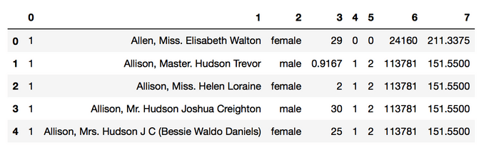
Studying the data frame you also see that we have a couple of infos for each passenger. In this case I took a look at the first entry:
- Passenger Class (1 = 1st; 2 = 2nd; 3 = 3rd)
- name (e.g. Allen, Miss. Elisabeth Walton)
- gender (e.g. female/male)
- age(e.g. 29)
- number of siblings/spouses aboard (e.g. 0)
- number of parents/children aboard (e.g. 0)
- ticket number (e.g. 24160) and
- passenger fare (e.g. 211.3375)
Step 2: Transform
As we expect that the ticket number is a string we can transcode it into a category. But since we don’t know which Ticket number Leo and Kate had, let’s just remove it as a feature. Similarly the name of a passenger in its form as a simple string is not going to be relevant either without preprocessing. To keep things short in this tutorial, we are simply going to remove both columns. We also want to dichotomize or label-encode the gender for each passenger mapping male to 1 and female to 0. Finally we want to transform the data frame back into a numpy float32 array, because that's what our network expects. To achieve those things I wrote a small function that works on a pandas dataframe does those things:
#Transform the data
def preprocess(r):
r = r.drop([1, 6], axis=1,errors='ignore')
r[2] = r[2].astype('category')
r[2] = r[2].cat.codes
for column in r.columns:
r[column] = r[column].astype(np.float32)
return r.values
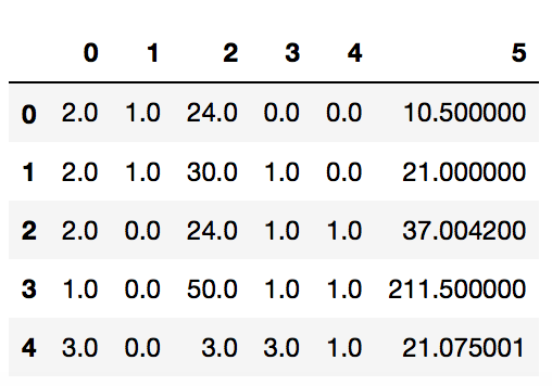
X_train = preprocess(X_train)
pd.DataFrame(X_train).head()We see that after the transformation the gender in the data frame is encoded as zeros and ones.
Step 3: Build the network
Now we can finally build our deep learning network which is going to learn the data. First of all, we specify the shape of our input data. The input sample has a total of 6 features, and we will process samples per batch to save memory. The None parameter means an unknown dimension, so we can change the total number of samples that are processed in a batch. So our data input shape is [None, 6]. Finally, we build a three-layer neural network with this simple sequence of statements.
net = tflearn.input_data(shape=[None, 6])
net = tflearn.fully_connected(net, 32)
net = tflearn.fully_connected(net, 32)
net = tflearn.fully_connected(net, 2, activation='softmax')
net = tflearn.regression(net)
If you want to visualize this network you can use Tensorboard to do so, although there will be not much to see (see below). Tensorflow won't draw all the nodes and edges but rather abstract whole layers as one box. To have a look at it you need to start it in your console and it will then become available on http://localhost:6006 . Make sure to use a chrome browser when you are looking at the graphs, safari crashed for me.
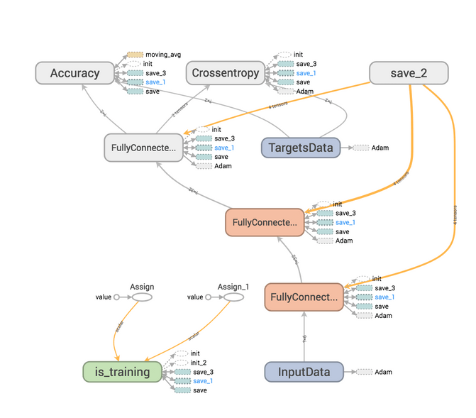
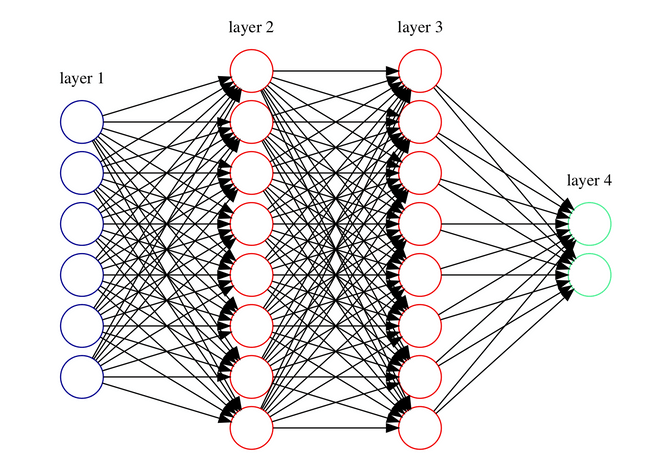
sudo tensorboard --logdir=/tmpWhat we basically have are 6 nodes, which are our inputs. These inputs are then connected to 32 nodes, which are then all fully connected to another 32 nodes, which are then connected to our 2 output nodes: one for survival, the other for death. The activation function softmax is the way to define when a node "fires". It is one option among among others like sigmoid or relu. Below you see a schematic I drew with graphviz based on a dot file, that you can download here . Instead of 32 nodes in the hidden layers I just drew 8, but you hopefully get the idea.
Step 4: Train it
TFLearn provides a wrapper called Deep Neural Network (DNN) that automatically performs neural network classifier tasks, such as training, prediction, save/restore, and more. I think this is pretty handy. We will run it for 20 epochs, which means that the network will see all the data 20 times with a batch size of 32, which means that it will take in 32 samples at once. We will create one model without cross validation and one with it to see which one performs better.
# Define model
model = tflearn.DNN(net)
# Start training (apply gradient descent algorithm)
model.fit(X_train, y_train, n_epoch=20, batch_size=32, show_metric=True)
# With cross validation if you want
model2 = tflearn.DNN(net)
model2.fit(data, labels, n_epoch=10, batch_size=16, show_metric=True, validation_set=0.1)
Step 4: Evaluate it
Well finally we've got our model and can now see how well it really performs. This is easy to do with:
#Evaluation
X_test = preprocess(X_test)
metric_train = model.evaluate(X_train, y_train)
metric_test = model.evaluate(X_test, y_test)
metric_train_1 = model2.evaluate(X_train, y_train)
metric_test_1 = model2.evaluate(X_test, y_test)
print('Model 1 Accuracy on train set: %.9f' % metric_train[0])
print("Model 1 Accuracy on test set: %.9f" % metric_test[0])
print('Model 2 Accuracy on train set: %.9f' % metric_train_1[0])
print("Model 2 Accuracy on test set: %.9f" % metric_test_1[0])
The output gave me very similar results for the train set (0.78) and the test set (0.77) for both the normal and the cross validated model. So for this small example the cross validation does not really seem to play a difference. Both models do a fairly good job at predicting the survival rate of the Titanic passengers.
Step 5: Use it to predict
We can finally see what Leonardo DiCaprio's (Jack) and Kate Winslet's (Rose) survival chances really were when they boarded that ship. To do so I modeled both by their attributes. So for example Jack boarded third class (today called the economy class), was male, 19 years old had no siblings or parents on board and payed only 5$ for his passenger fare. Rose traveled of course first class, was female, 17 years old, had a sibling and two parents on board and paid 100$ for her ticket.
# Let's create some data for DiCaprio and Winslet
dicaprio = [3, 'Jack Dawson', 'male', 19, 0, 0, 'N/A', 5.0000]
winslet = [1, 'Rose DeWitt Bukater', 'female', 17, 1, 2, 'N/A', 100.0000]
# Preprocess data
dicaprio, winslet = preprocess([dicaprio, winslet], to_ignore)
# Predict surviving chances (class 1 results)
pred = model.predict([dicaprio, winslet])
print("DiCaprio Surviving Rate:", pred[0][1])
print("Winslet Surviving Rate:", pred[1][1])
The output gives us:
- DiCaprio Surviving Rate: 0.128768
- Winslet Surviving Rate: 0.903721
Conclusion, what's next?
So after all we know it was a rigged game. Given his background DiCaprio really had low chances of surviving this disaster. While we didn't really learn anything new about the outcome of the movie, I hope that you enjoyed this quick intro into Tensorflow and Tflearn that are not really hard to get into and don't have to end with a disaster.
In our example there was really no need to pull out the big guns, a simple regression or any other machine learning method would have worked fine. Tensorflow, TFlearn or Keras really shine though when it comes to Image, Text and Audio recognition tasks. With the very popular Keras library we are almost able to reduce the boilerplate for these tasks even more, which I will cover in one of the future blog posts. In the meantime I encourage you to play around with neural networks in your browser in this excellent examples and am looking forward for your comments and hope that you enjoyed this little fun blog post. If you want you can download the Ipython notebook for this example here .