

Business Problem
Time Series prediction can be used in a number of business areas. You can think of a number of areas and questions. For example
- Marketing/Sales: How are our sales numbers going to be in Q4?
- Health: Do we need more beds in the hospital next year?
- Sports: When is the outdoor pool temperature finally going to reach 21°C this year?
- Sales: Will we sell enough watches this year to make the target we have set?
- Energy: What will the energy consumption of this household be tomorrow?
Generally, a prediction problem involves using past observations to predict or forecast one or more possible future observations. The goal is to guess about what might happen in the future. Knowing the future can impact our decisions today so we have a great interest in predicting it. So in this blog article I want to show you a couple of techniques that you might try and provide you with a couple of tools that you can try right away.
This blog post was heavily inspired by the book “Deep Learning for Time Series Forecasting - Predict the Future with MLPs, CNNs and LSTMs in Python” from Jason Brownlee who did an excellent job summarizing all of the approaches and methods in one big 700 pages book. If you feel you want to deep dive into time series prediction make sure give it a try.
Challenges
Generally when predicting time series there are a number of challenges that are specific for this set of problems:
- In a time series, the observations for an input variable depend upon one another. For example, the observation at time t is dependent upon the observation at t−1; t−1 may depend on t−2, and so on. We call such variables endogenous because it is affected by other variables in the system and the output variable depends on it. Although time series might also have exogenous variables (variables that are not influenced by other variables) it's usually these endogenous property of variables that distinguishes them from other problems.
- Time series may have obvious patterns, such as a trend or seasonal cycles.
- Sometimes we just want to predict the next time step, but sometimes we might even want to predict multiple steps, which makes our prediction harder.
- Additionally some models age well over time, thus meaning they are “static” and have not to be updated, while others are dynamic, e.g. you have to retrain your model every week.
To make things even harder sometimes we have contiguous data, meaning that we have uniform observations over time, but more often than not we have discontinuous data, where the observations are not uniform over time and so needs additional preparation.
Choosing a framework to work with
Generally there are a number of different approaches to predicting time series, some of them are able to reflect the number of different challenges while others are not. Thus it totally depends on your problem what the right choice is. Let's dive in.
Usually you already have your dataset (a database, csv, etc..) and you know what needs to be forecasted and maybe you even have a clue how to evaluate a model that you have built. The fastest and most secure way forward from my experience is to start with easy models and make your way up to the more complex ones, in order to figure out if you are making any progress. So we will be following occam's razor which says: one should select the solution with the fewest assumptions.
So our progression in this blog post will look like the following:
- Make a simple baseline e.g. average the data
- Try autoregression e.g. SARIMA models (Seasonal Autoregressive Integrated Moving Average Models)
- Try exponential smoothing e.g. smooth the s*** out of the data, but this time use explicitly exponential functions not linear
- Try a simple neural network
- Try deep learning CNN, LSTM, etc..
Now you are probably reading this because you want to know how number 5 works, but more often than not you really don’t need a deep learning model, often just having number 1 through 3 gives you enough precision to support your business.
Of course if precision is your big goal then trying the complicated models may be worth your time, otherwise not. We will cover all techniques except for number 5, which we will cover explicitly in the next blog post of this series.
Yet, let me first present you with a couple of useful concepts that help us train, test, tune and evaluate our models. I will only cover here the simplest way aka predicting the next step in time series. So for example if you have daily data, this means we just look one day ahead. If you predict multiple days ahead you will need slightly different ways to test the data, but the rough idea stays the same.
How to train our models?
Generally in machine learning we split the data into train and test in order to see how well our model performs, but time series data is kind of special because it has an ordering. Thus we have to write a split function that maintains this ordering while taking a number of ordered observations. So we are not splitting our data by random but instead we leave the ordering and just take chunks of data for training and testing.
# split the train and test data, maintaining the order
def train_test_split(data, n_test):
    return data[:-n_test], data[-n_test:]
How to test our models?
After having fitted the model (see below) we want to make a forecast for the given history, then compare the prediction to the actual value that was going to come next. For this we can use the root mean squared error, which is a pretty standard way of measuring errors in machine learning.
# measure the root mean squared error
def measure_rmse(actual, predicted):
    return sqrt(mean_squared_error(actual, predicted))
So to test how our model works not just for one data point but the whole points contained in the test data, we have to split our model multiple times, each time adding one datapoint to the training data and seeing what the model will predict. This way of constantly splitting the data and looking ahead is called walk forward validation.
# walk forward validation in a step by step manner
def walk_forward_validation(data, n_test):
    predictions = list()
    train, test = train_test_split(data, n_test)
    model = model_fit(train)
    history = [x for x in train] #seed history with training data
      # walk forward
    for i in range(len(test)):
        # fit model and make forecast for history
        yhat = model_predict(model, history)
        predictions.append(yhat) #store the forecast
        history.append(test[i]) #add it to history for next loop
    # estimate error
    error = measure_rmse(test, predictions)
    print(' > %.3f' % error)
How to tune our models?
Since the methods that we will try depend heavily on a number of hyperparameters (e.g. how many seasons does a year have, do we want to average over the last 3,4,5 or 10 data points, …) we cannot know which hyperparameters are going to give us the best result. For this one way of approaching the problem can be to simply try all of the combinations and see which ones work best on the test data. This is also called a grid search.
A simple example would be: for the average baseline model try averaging over the last 1,2,3, … all values in the dataset and see which n returns the best results. So here we have one hyperparameter. In other models we might have to tweak multiple parameters to find which combination works best.
Lets predict something!
To see how well our models do we can test them on 4 different datasets.
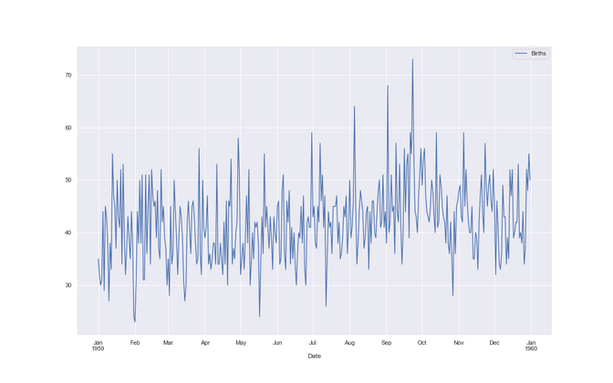
Female births in California in 1959

The first dataset has almost no “trend” - which means that the numbers are roughly not going up or down over a longer period. In our case the dataset is called “female births in California in 1959”. Regarding the business case, we can easily think how it would be good to know the next years numbers in order to know if we need more staff, or more beds, so we don’t run out of capacity and can offer a good service. One step is one day in this dataset.
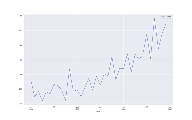
Shampoo sales over a three year period

The second dataset has a “trend”. Its called https://www.kaggle.com/guangningyu/sales-of-shampoo sales of shampoo over a three year period. We can clearly see that this company is selling more and more shampoo each year, so they better should know ahead how much they are going to sell next year in order to be able to plan ahead nicely. One step is one month.
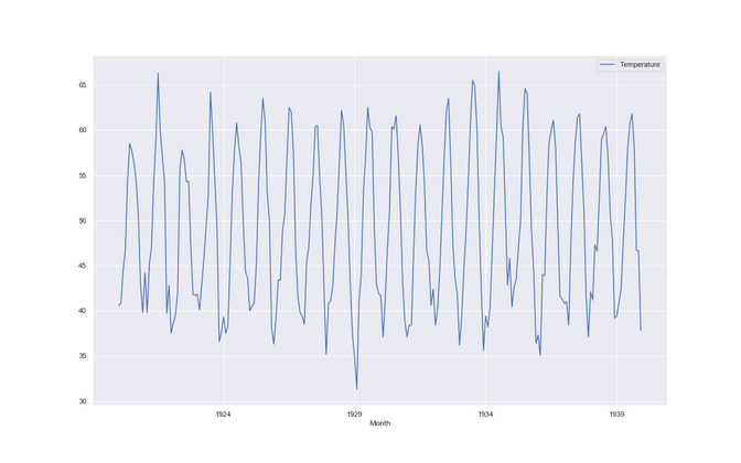
Average monthly temperature over three years

The third dataset has no trend but a new thing called seasonality. It is called monthly average temperature over three years. Here we can roughly say we don’t see an average rise in temperature, but it seems to fluctuate a lot during the year in a regular way aka. it's hot in the summer and cold in the winter - what a surprise :). We might think of a business case where an ice cream factory needs to know when it needs to ramp up their production in order to not run out of stock. One step is one month.
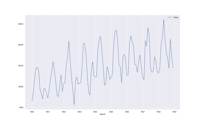
Car sales in quebec in the 60ties

The fourth dataset has seasonality and a trend. Its called monthly car sales in quebec in the 60ties. We see that although on average the number of car sales is going up over the years, the sales also depend a lot on the season of the year. It seems that people love to buy their cars in spring and autumn. One step is one month.
After having introduced the datasets let us dive into the methods.
1. Baseline average
One of the simplest things that we can try is to take the n-last value from the data and simply do a median or mean on this subset. Depending on the n we are either taking into consideration a long or short history.
# use mean or median to predict the future
def average_forecast(history, config):
n, avg_type = config
if avg_type is 'mean':
return mean(history[-n:])
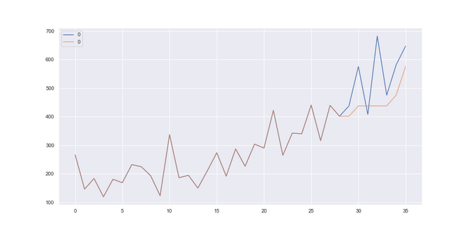
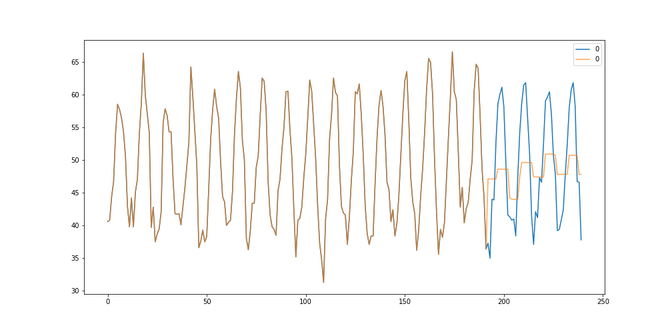
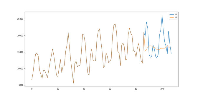
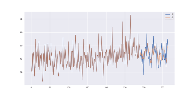
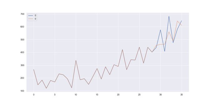
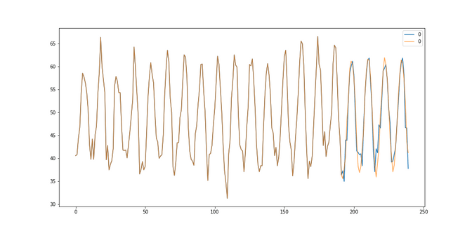
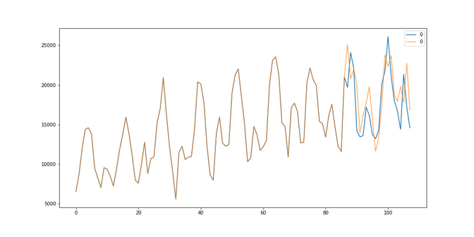
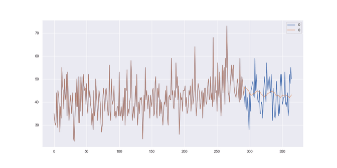
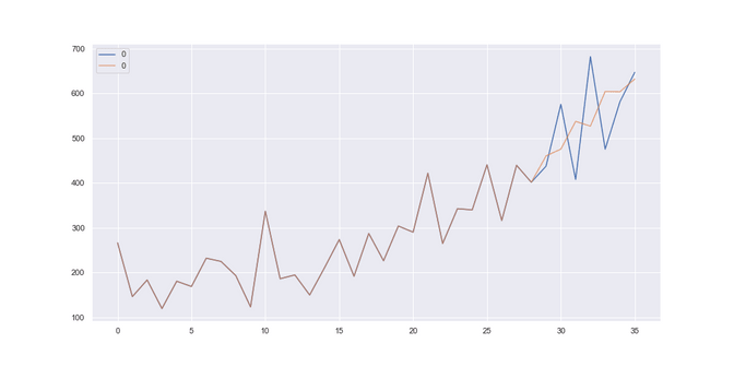
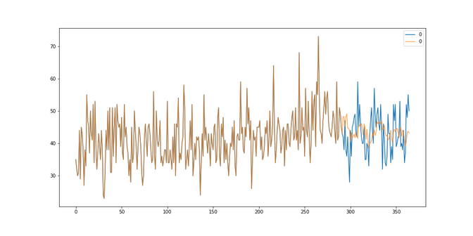
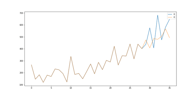
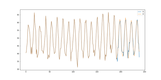
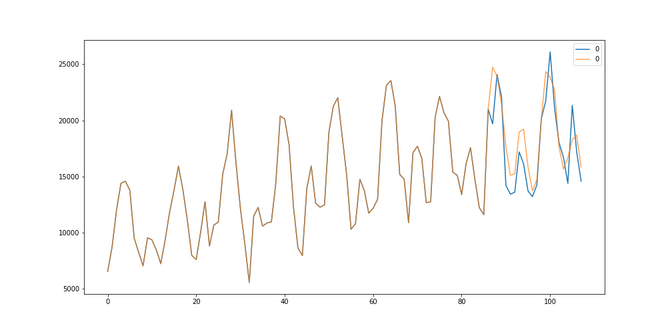
return median(history[-n:])Although this model looks a bit “stupid” it might do the job well for data where there is a lot of noise, are where we want to put a strong emphasis only on the last values. So how does it do on our datasets? Let's have a look: The brown line is the history that we trained it on, the blue line is the “future” and the orange line is the prediction of our model.
Female births: It got the best results, aka it got the lowest RMSE of 6.37, when it was looking back on the last 192 days and used a mean to average the history. Although our prediction does not model all the peaks of the data, at least it seems to get that the data doesn’t change much, so it predicts the same value every time.

Shampoo sales: Here we got the best results looking back at the last 2 months, using a median and our RMSE was 113. Our model seems to somehow doing ok, it simply sticks to rather new data and is able to keep up with the trend somehow.
Temperature: Here we got the best results looking back 1 months using a median strategy. Our RMSE was 5.14. We see that our average strategy seems to be lagging behind the actual data and it is.
Car Sales: Here we got the best results looking back 1 months using a median strategy. The RMSE was 3647. We see that somehow our average strategy simply relies on sticking to the present. Another good result is also obtained with a mean of 14 days, resulting in a RMSE of 4085.
2. SARIMA models
The next family of models we are going to look at are the SARIMA (Seasonal Autoregressive Integrated Moving Average) models. You can very easily use them because they come in the form of a library that can be imported directly from statsmodels. It has basically three different parameter-types:
- Order: A tuple p, d, and q parameters for the modeling of the trend. They control the order of the autoregression, of the difference and of the moving average.
- Seasonal order: A tuple of p,d, q, and m parameters for the modeling the seasonality. These also control the order of the seasonal autoregression, seasonal difference, seasonal moving average and the number of steps that contribute towards one seasonal period.
- Trend: A parameter for controlling a model of the deterministic trend. It can either be ‘n’, ‘c’,‘t’, and ‘ct’ for: no trend, constant, linear, and constant with linear trend, respectively.
If we know enough about the problem we might specify them correctly or we can just try to grid-search them. We will just do this as we did for the average models. We see below that we can supply these parameters fit the model and then use it to predict the results for the next step.
# A simple way to use SARIMAX from statsmodels
def sarima_forecast(history, order, sorder, trend):
    model = SARIMAX(history, order=order, seasonal_order=sorder, trend=trend,
      enforce_stationarity=False, enforce_invertibility=False)
    # fit model
    model_fit = model.fit(disp=False)
    # make one step forecast
    yhat = model_fit.predict(len(history), len(history))
    return yhat[0]
So how does this model do on our data?
Female births: It seems to have picked up a small pattern in the data, with a RMSE of 6,16 so it actually improved on the baseline method.
Shampoo sales: For the shampoo sales we see that the model picked up the trend very nicely. The best parameters resulted in a RMSE of 62.8 so a big improvement against the baseline of 113 in the average model.
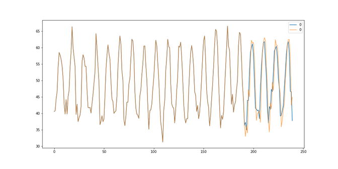
Temperature: Here we see an almost perfect fit in the data, notice how nicely the orange (predicted) curve matches the blue (actual data) one. This results in a RMSE of 2.27 so a big improvement on the 5.14 of the baseline model.
Car sales: Here we see nicely how the best fitting SARIMA model picked up the trend and seasonality. This results in a RMSE of 2600 vs the 3647 in the baseline model. So quite an improvement.
We see that the family of SARIMA models is very capable to model different types of time series, each time hugely improving on the baseline of simply going with an average. Let’s find out if the exponential smoothing can improve on this.
3. Exponential Smoothing or Winter-Holt models
Exponential smoothing models are a time series forecasting method for univariate data. While in the SARIMA models the prediction is simply a weighted linear sum of recent past observations, in exponential smoothing the model explicitly uses an exponentially decreasing weight for past observations. Specifically, past observations are weighted with a geometrically decreasing ratio.
There are basically three types of exponential smoothing time series forecasting methods. A simple method that assumes no systematic structure, an upgrade that explicitly handles trends, and the most advanced method that has additionally support for seasonality. We will use the most advanced model in our forecast.
The implementation from statsmodels already has an optimizer that automatically tunes these hyperparameters for us: the smoothing coefficient for the level (alpha), the smoothing coefficient for the trend (beta), the smoothing coefficient for the seasonal component (gamma) and the coefficient for the damped trend (phi).
Yet we need to grid search these parameters:
- trend (t): The type of trend component, as either add for additive or mul for multiplicative. It can also be set to None.
- damped(d): Whether or not the trend component should be damped, either True or False.
- seasonality(s): The type of seasonal component, as either add for additive or mul for multiplicative. It can be turned off with None.
- seasonal periods (p): The number of time steps in a seasonal period, e.g. 12 for 12 months in a yearly seasonal structure.
- boxcox(b): Whether or not to perform a power transform of the series.
- Remove bias(r): If the bias/trend should be removed from the data
# Exponential smoothing with statsmodels
def exp_smoothing_forecast(history, t,d,s,p,b,r):
    history = array(history)
    model = ExponentialSmoothing(history, trend=t, damped=d, seasonal=s, seasonal_periods=p)
    # fit model
    model_fit = model.fit(optimized=True, use_boxcox=b, remove_bias=r)
    # make one step forecast
    yhat = model_fit.predict(len(history), len(history))
    return yhat[0]
So how does this family of models do on our data?
Female-births: Well here we are rather closer to the solution that the average baseline offered us. Apparently the models didn’t pick up on the fluctuations, which results in a RMSE of 6,74 which is the worst of all models so far.
Shampoo sales: Here the prediction looks better although I feel like it has a certain lag. This can be taken care of with additional modeling but with an RMSE of 97 we are a little bit better than the average model but worse than the SARIMA model.
Temperature: Here we got quite a mediocre fit to the data. The RMSE of 4.57 is much worse than the 2.45 of the SARIMA models and only slightly better than the baseline.
Car sales: The fit to the care sales looks pretty good although we also have this “lag” problem here. With a RMSE of 3635 we are quite a bit worse than the SARIMA solutions.
Little Mid-Resume
Based on our little experiments so far we see that the average models seem not to be so bad in comparison to the much more complicated models. Yet the Winter-Holt models seem to do worse than the SARIMA models, which have shown a very good performance, given that they had so little training data (e.g. often only less than 100 data points).
4. Neural networks
Before we can try different methods, we have to re-shape our data a little bit to make it work with normal machine learning methods.
Time series as a supervised learning problem
While we can use special methods that work on time-series data only we can also re-frame time series as a simple supervised learning problem. We go from representing the data like this:
| time | measure |
|---|---|
| 1 | 100 |
| 2 | 110 |
| 3 | 108 |
| 4 | 115 |
| 5 | 120 |
To this:
| X | y |
|---|---|
| ? | 100 |
| 100 | 110 |
| 110 | 108 |
| 108 | 115 |
| 115 | 120 |
| 120 | ? |
Doing this is called a window approach or a lag method. The number of previous states is the window size or lag, so in our example above 1. The benefit is that now we can work with any linear or nonlinear standard ml method giving us more flexibility in our toolkit. In code it looks like this - using the pandas shift method we can copy and shift the data next to each other.
# Transforming time-series to a supervised problem
def series_to_supervised(data, n_in, n_out=1):
    df = DataFrame(data)
    cols = list()
    # input sequence (t-n, ... t-1)
    for i in range(n_in, 0, -1):
        cols.append(df.shift(i))
    # forecast sequence (t, t+1, ... t+n)
    for i in range(0, n_out):
        cols.append(df.shift(-i))
    # put it all together
    agg = concat(cols, axis=1)
    # drop rows with NaN values
    agg.dropna(inplace=True)
    return agg.values
So for our example of car sales this method would produce the following results:
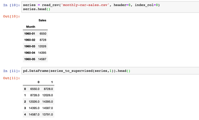
Now we can write the forecast using a simple neural network with keras.
# Fit a NN model
def neural_network_forecast(history, n_input,n_nodes,n_epochs,n_batch):
    data = series_to_supervised(history, n_input)   # prepare data
    train_x, train_y = data[:, :-1], data[:, -1] # first col input, last pred
    # define model
    model = Sequential()
    model.add(Dense(n_nodes, activation='relu', input_dim=n_input))
    model.add(Dense(1))
    model.compile(loss='mse', optimizer='adam')
    # fit
    model_fit = model.fit(train_x, train_y, epochs=n_epochs, batch_size=n_batch, verbose=0)
    x_input = array(history[-n_input:]).reshape(1, n_input)
    # make one step forecast
    yhat = model.predict(x_input, verbose=0)
    return yhat[0]
We are basically doing the same as above, with the added step that we transform the data in the way described above. The neural network is modeled with keras where we have one Dense layer that takes the input that is connected to one dense layer that is the output of our model. We can experiment with the number of data points that we look at at the same time (e.g. 12/24) the number of nodes that our network has (e.g. 50/100/500…), number of epochs (e.g. 100) and the batch size (e.g 100).
So how does it do on our data?
Female Births: We see that the model picked up quite a bit of the fluctuations, giving us a RMSE of 6.7 . Yet this is not better than the baseline and the SARIMA models.
Shampoo sales: We did quite bad on the shampoo sales. We got a RMSE of 115, so not even an improvement against the baseline and much worse than the SARIMA (RMSE 62) models and somewhere similar than the Winter Holt models (RMSE 97)
Temperature: With a RMSE of 2.20 we have even managed to beat the results of the SARIMA models (2.27) which is a nice surprise!
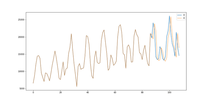
Car sales: With a RMSE of 2091 we did excellent modeling a trend and seasonality. We have outperformed the SARIMA models (RMSE 2600) by quite a bit.
So there you have it, apparently our very simple neural network wasn’t best in all categories, but it managed to give us a great performance for the temperature seasonal time series and the trend+seasonal time series when modeling the car sales.
Summary
Given our little contest we can draw the following table below. We see that SARIMA ant the simple neural network gave us the best results for our small examples. This should not lead you to the conclusion that you should only use these methods and forget the rest, but instead, that it's worth trying them all. We might for example notice that a simple average does pretty well sometimes (e.g. for the female births) and that it might not be worth it to add that much complexity in order to improve just a few percent.
| No-Trend | Trend | Seasonality | Trend+Seasonality | |
|---|---|---|---|---|
| Dataset / Method | Female births | Shampoo Sales | Temperature | Car Sales |
| Average | 6,37 | 113,15 | 5,14 | 3647 |
| SARIMA | 6.16 (WINNER) | 62.83 (WINNER) | 2,27 | 2600 |
| Holt-Winters | 6,74 | 97 | 4,57 | 3635 |
| Simple Neural-Network | 6,7 | 115 | 2.20 (WINNER) | 2091 (WINNER) |
Time Series prediction out of the box
Aaaand one more thing - If you are still here, it seems I might as well share with you one secret that will make your life easier when working with time series. There is a very nice library called Prophet out there, that makes predicting time series an almost effortless endeavour. Apparently the engineers at Facebook were tired to reinvent the wheel every time they “just” needed to predict some data into the future. So they’ve built their own open source tool.
“Prophet is a procedure for forecasting time series data based on an additive model where non-linear trends are fit with yearly, weekly, and daily seasonality, plus holiday effects. It works best with time series that have strong seasonal effects and several seasons of historical data. Prophet is robust to missing data and shifts in the trend, and typically handles outliers well.”
Let me show you how it works. First you need to whip the data a little bit into shape, by giving it the right column names and types and then you are basically ready to go.
# A few simple preprocessing steps
series = pd.read_csv('monthly-car-sales.csv', header=0, index_col=None)
series['ds']  = pd.to_datetime(series['Month'])
series[['y']] = series[['Sales']].astype(float)
series = series[["ds","y"]]
series.head()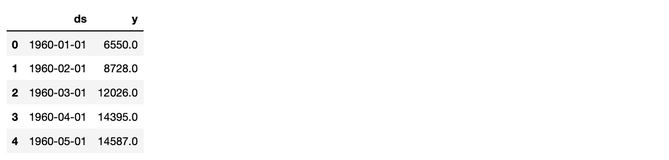
Then you supply it with the most important parameters: which is the number of periods it should predict and what the frequency of your data is (e.g. months) . You select a seasonality mode and can also add different seasonalities for weeks, months, etc… and then fit the data.
# A simple prediction
m = Prophet(mcmc_samples=500,seasonality_mode='multiplicative').fit(series);
future = m.make_future_dataframe(periods=48,freq='M')
forecast = m.predict(future)
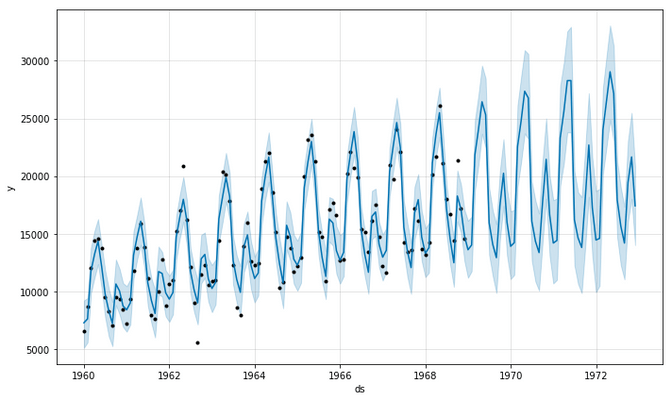
forecast[['ds', 'yhat', 'yhat_lower', 'yhat_upper']].tail()The outcome is a model that can predict your data not only one step into the future but multiple. Of course each step will have more uncertainty in it. We can as well do this with our methods above, I am just saying that with prophet it already comes in the box, which is a nice thing. So how does a prediction look like? Let's have a look at the car sales.
Below you see a standard output from prophet, where it shows us the data points in black and the prediction in blue. It even shows us the rising uncertainty in the future (light blue)
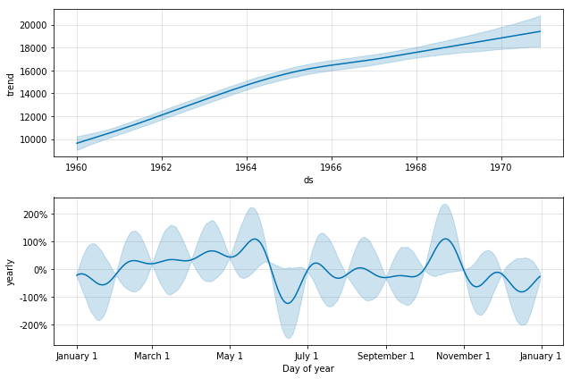
We also get the trend and seasonal components right out of the box, where we can investigate that car sales happen mostly around spring and autumn, but less in the hot summer days.
So how does it do vs the other methods?
We will even be a bit unfair and just see how well the multi-step predictions of prophet match up with the one-step predictions we have used before.
| No-Trend | Trend | Seasonality | Trend+Seasonality | |
|---|---|---|---|---|
| Dataset / Method | Female births | Shampoo Sales | Temperature | Car Sales |
| Best Method | 6.16 (SARIMA) | 62.83 (SARIMA) | 2.2 (Neural Network) | 2091 (Neural Network) |
| Prophet | 6,64 | 37,67 | 1,91 | 1382 |
It turns out Prophet has beaten almost all of our simple methods by quite a bit. So should we always just use prohphet and forget the rest? Well it still depends. If you need something where you quickly get a prediction then use prophet. If you need to have influence over the method or want to have a prediction more sophisticated than our simple examples then you should invest the time into modeling it yourself.
Also when it comes to a multivariate prediction you might be better of using your own method although prophet might also work using the VAR method
Summary
So what’s the lesson here? Maybe we have a couple:
- If you want to predict time series, start simple and a simple method might just be enough.
- If you add complexity, then measure if it was worth it.
- When working with more complex methods, you can gridsearch the solution although it is rather costly.
- You have multiple options on which methods to use, including more recent machine learning methods like deep learning.
- If you need something out of the box, for a simple univariate time series libraries like prophet might be just right to do the job.
That's it folks! You can find the code that was used to generate these time series prediction as usual in our GitHub repo.